非日数据

次日数据

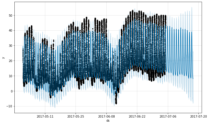
Prophet can make forecasts for time series with sub-daily observations by passing in a dataframe with timestamps in the ds column. The format of the timestamps should be YYYY-MM-DD HH:MM:SS - see the example csv here. When sub-daily data are used, daily seasonality will automatically be fit. Here we fit Prophet to data with 5-minute resolution (daily temperatures at Yosemite):

Prophet可以通过在 ds列中传递一个带有时间戳(timestamps)的dataframe ，对具有次日观测的时间序列进行预测。时间戳的格式应该是YYYY-MM-DD HH:MM:SS–请看示例csv这里。当使用次日数据时，每日的季节性将被自动拟合。这里，我们将用Prophet拟合5分钟频率的数据（Yosemite的日气温）。

# Rdf <- read.csv('../examples/example_yosemite_temps.csv')m <- prophet(df, changepoint.prior.scale=0.01)future <- make_future_dataframe(m, periods = 300, freq = 60 * 60)fcst <- predict(m, future)plot(m, fcst)

# Pythondf = pd.read_csv('../examples/example_yosemite_temps.csv')m = Prophet(changepoint_prior_scale=0.01).fit(df)future = m.make_future_dataframe(periods=300, freq='H')fcst = m.predict(future)fig = m.plot(fcst)

png

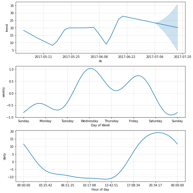
每日的季节性将在成分图中显示出来。

# Rprophet_plot_components(m, fcst)

# Pythonfig = m.plot_components(fcst)

png

带有规律空白的数据

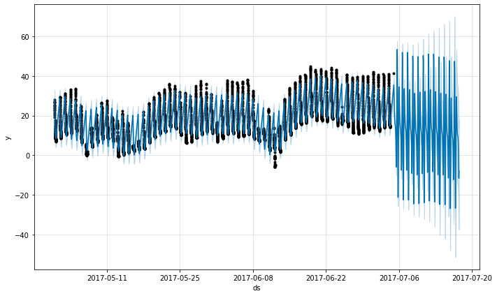
假设上述数据集只有12a至6a的观测值。

# Rdf2 <- df %>%  mutate(ds = as.POSIXct(ds, tz="GMT")) %>%  filter(as.numeric(format(ds, "%H")) < 6)m <- prophet(df2)future <- make_future_dataframe(m, periods = 300, freq = 60 * 60)fcst <- predict(m, future)plot(m, fcst)

# Pythondf2 = df.copy()df2['ds'] = pd.to_datetime(df2['ds'])df2 = df2[df2['ds'].dt.hour < 6]m = Prophet().fit(df2)future = m.make_future_dataframe(periods=300, freq='H')fcst = m.predict(future)fig = m.plot(fcst)

png

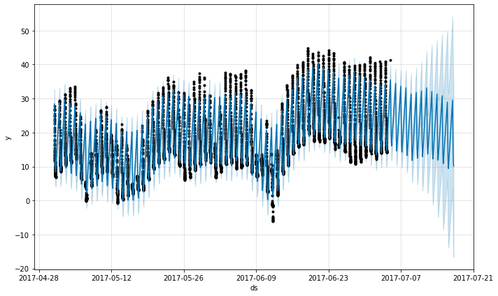
预测似乎相当糟糕，未来的波动比历史上看到的要大得多。这里的问题是，我们将一个日周期拟合到一个时间序列上，而这个时间序列只有一天中部分时间（12a至6a）的数据。因此，每日的季节性对一天中剩余的时间没有限制，不能很好地估计。解决办法是只对有历史数据的时间窗口进行预测。在这里，这意味着将 “未来”数据框架的时间限制在12a至6a之间。

# Rfuture2 <- future %>%  filter(as.numeric(format(ds, "%H")) < 6)fcst <- predict(m, future2)plot(m, fcst)

# Pythonfuture2 = future.copy()future2 = future2[future2['ds'].dt.hour < 6]fcst = m.predict(future2)fig = m.plot(fcst)

png

同样的原则也适用于数据中存在规律性空白的其他数据集。例如，如果历史记录只包含工作日，那么只能对工作日进行预测，因为周末的周季节性将不能很好地估计。

月度数据

You can use Prophet to fit monthly data. However, the underlying model is continuous-time, which means that you can get strange results if you fit the model to monthly data and then ask for daily forecasts. Here we forecast US retail sales volume for the next 10 years:

# Rdf <- read.csv('../examples/example_retail_sales.csv')m <- prophet(df, seasonality.mode = 'multiplicative')future <- make_future_dataframe(m, periods = 3652)fcst <- predict(m, future)plot(m, fcst)

# Pythondf = pd.read_csv('../examples/example_retail_sales.csv')m = Prophet(seasonality_mode='multiplicative').fit(df)future = m.make_future_dataframe(periods=3652)fcst = m.predict(future)fig = m.plot(fcst)

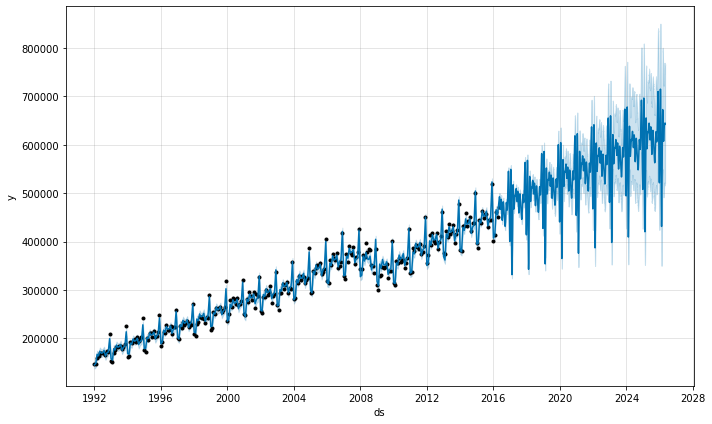
png

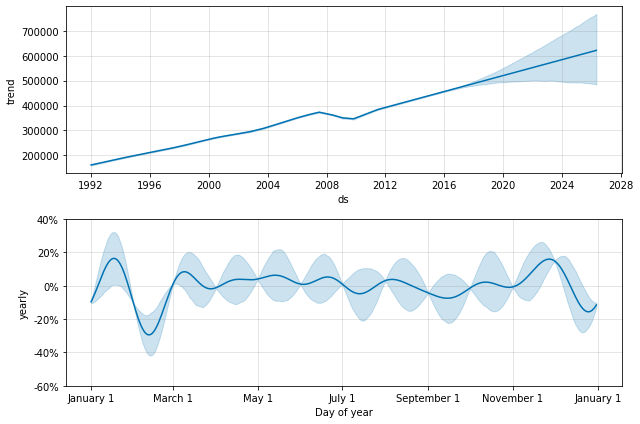
这和上面的问题是一样的，数据集有规律的空白。当我们拟合年度季节性时，它只有每个月1号的数据，其余天数的季节性分量是无法识别和过拟合的。这一点可以通过做MCMC来清楚地看到季节性的不确定性。

# Rm <- prophet(df, seasonality.mode = 'multiplicative', mcmc.samples = 300)fcst <- predict(m, future)prophet_plot_components(m, fcst)

# Pythonm = Prophet(seasonality_mode='multiplicative', mcmc_samples=300).fit(df)fcst = m.predict(future)fig = m.plot_components(fcst)

WARNING:pystan:403 of 600 iterations saturated the maximum tree depth of 10 (67.2 %)
WARNING:pystan:Run again with max_treedepth larger than 10 to avoid saturation

png

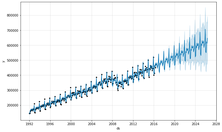
在每个月开始有数据点的地方，季节性的不确定性很低，但中间的后方差非常高。在对月度数据拟合Prophet时，只做月度预测，可以通过将频率传入make_future_dataframe来实现。

# Rfuture <- make_future_dataframe(m, periods = 120, freq = 'month')fcst <- predict(m, future)plot(m, fcst)

# Pythonfuture = m.make_future_dataframe(periods=120, freq='MS')fcst = m.predict(future)fig = m.plot(fcst)

png

在Python中，频率可以是这里的pandas频率字符串列表中的任何内容：https://pandas.pydata.org/pandas-docs/stable/user_guide/timeseries.html#timeseries-offset-aliases 。请注意，这里使用的 “MS”是月份开始，意味着数据点被放在每个月的开始。

在月度数据中，年度季节性也可以用二元额外回归因子来建模。特别是，该模型可以使用12个额外的回归因子，如 is_jan、is_feb等，其中 is_jan如果日期在1月，则为1，否则为0。这种方法可以避免上面看到的月内无法识别的情况。如果要添加月度额外的回归因子，一定要使用yearly_seasonality=False。

有汇总数据的假日

假日效应适用于指定假日的特定日期。对于已经汇总为周或月频率的数据，不属于数据中使用的特定日期的假日将被忽略：例如，在每周时间序列中，每个数据点都在周日的周一假期。要在模型中包含假日效应，需要将假日移到历史数据框架中需要该效应的日期。需要注意的是，对于每周或每月的汇总数据，许多假日效应将被年度季节性所充分体现，因此只有在整个时间序列的不同星期发生的假日才需要增加假日。